Renderer written in C++ with support for global illumination and physically-based materials.

Overview

In this project, I built a raytracer that can trace paths of light through a scene in order to render 3D scenes with realistic lighting. I implemented ray generation, primitive intersections, bounding volume hierarchy (BVH) intersections, direct lighting with uniform hemisphere sampling and importance sampling on lights, indirect lighting with recursive raytracing and, finally, adaptive sampling.

Overall, I spent a while optimizing my intersection tests so that I could generate renders locally in a reasonable amount of time. A lot of my debugging time was focused on implementing direct and indirect lighting, since small errors such as numerical imprecision or incorrectly converted values had noticeable effects on the final renders. As a 3D artist who works frequently with rendering software such as Pixar’s RenderMan, working through this project gave me a better understanding of the math behind it all. While I knew about these sampling definitions and the general concepts behind rendering, coding these different parts of global illumination allowed me to better conceptualize how all these rendering parameters affect the pathtracer.

Part 1: Ray Generation and Intersection

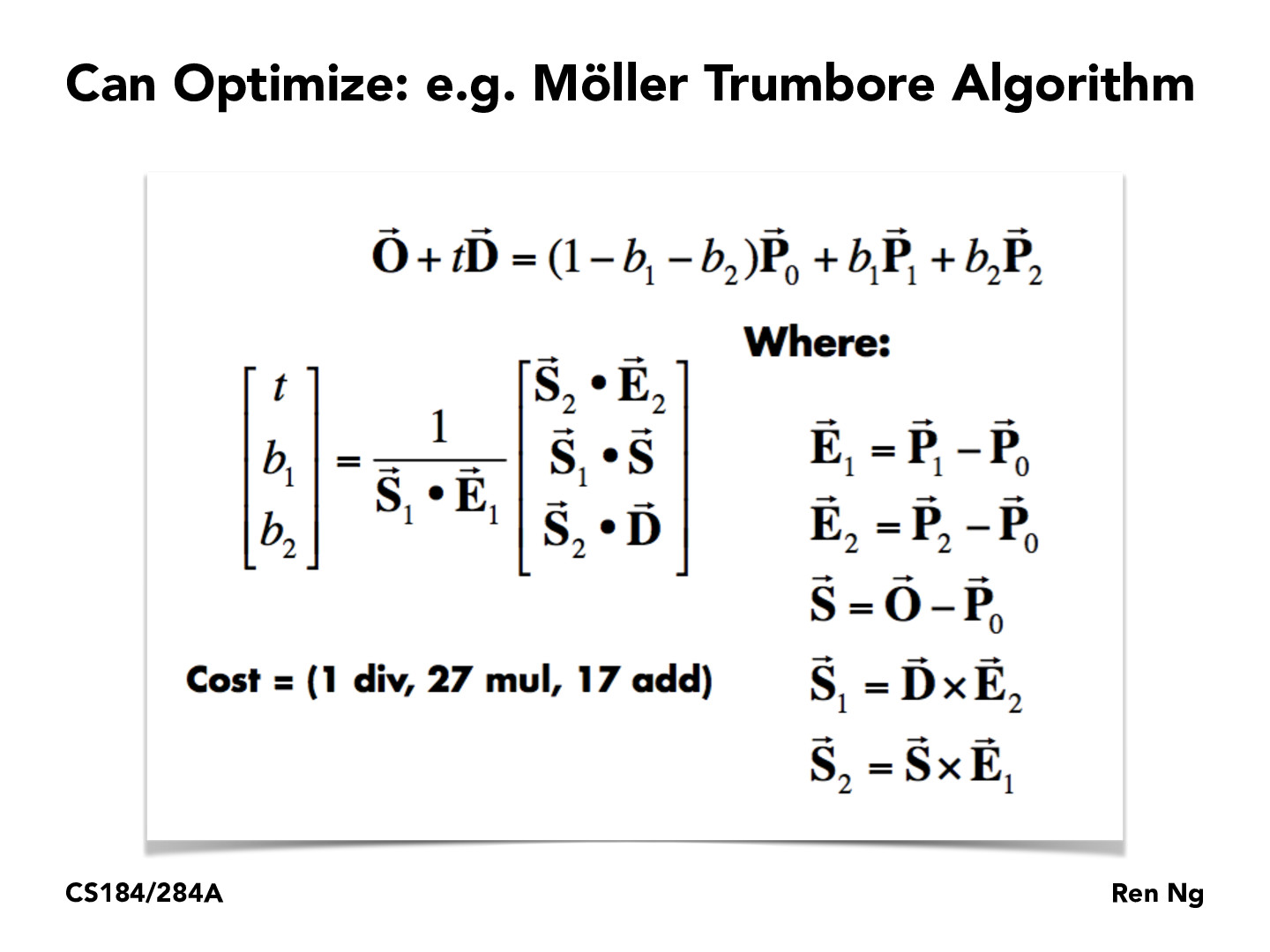
In order to begin raytracing, rays must be generated from the camera for each pixel of the image space to explore visible objects. These rays must also be able to intersect with primitives and return a color (Spectrum) value, which will get averaged with the values returned sample rays for the same pixel to get the final color for that pixel. The primitives supported by this raytracer are triangles. I used the Möller-Trumbore ray-intersection algorithm to find the t value for which the ray intersects with a primitive.

The Möller-Trumbore algorithm solves for the barycentric coordinates of the ray on the plane defined by the current triangle, allowing us to check if the ray is within the triangle. Below are some examples of normal shading for a few different DAE files.

Part 2: Bounding Volume Hierachy

My BVH algorithm processes every primitive and saves the coordinates of each primitive’s centroid, computing the average of all centroids at the end of the loop. Based on which axis (x, y, or z) has the greatest range of values, the primitives are split depending on if they lie on the left or right of the average of all centroids in the axis of greatest range. This algorithm runs quite quickly and produces a pretty good hierarchy for scenes that can be easily divided into left/right binary components.

Below are a few DAE files that would take much longer to render without the BVH structure in place.

The cow was moderately complex to the point that it could still render without the BVH in place. Without the BVH, rendering the cow with normal shading took 49.1854s. After implementing my BVH, it rendered in only .5541s. CBlucy, which has hundreds of thousands of triangles, rendered even faster at .3751s, while maxplanck took 0.6468s to render. In general, the complexity of the scenes no longer had a huge effect on the runtime of the rendering process, which makes sense since the purpose of the BVH is to make the runtime logarithmic with respect to the input size.

Part 3: Direct Illumination

Direct lighting was implemented in two different ways: uniform hemisphere sampling and importance sampling on lights. Both methods are preceded by calculating the zero bounce radiance, which are the samples of camera rays that directly hit light sources. For rays that instead intersect with objects in the scene, the ray and the intersection information are passed to the direct lighting functions. For uniform hemisphere sampling, my code generates secondary rays according to the number passed in by the rendering parameters. Each of these secondary rays start at the intersection point of the camera ray in the world space. The direction for these rays is randomly sampled from a uniform distribution. Next, my code traces the path of the current secondary ray and tests if it intersects with a light by looking at the emission of the returned intersection object. If the bounce does reach a light, then I add the contribution from this bounce to the output, with the incoming light taken from the light’s emission value. After all secondary rays have finished being evaluated, I normalize by the number of samples taken and return the light value for this sample ray.

For importance sampling on lights, the code once again takes in a sample ray and the intersection data for this sample ray. My implementation then loops through each light in the scene’s lights vector. If the current light being sampled from is a point light, my code samples only one direction instead of num_samples, since there is only one possible path from a point light to an intersection point. For area lights, I loop again to sample from different parts of the area light. Unlike uniform hemisphere sampling, the intersection test is only done to check if the secondary rays are occluded on their path to the light–in other words, the path tracing is done to determine if the current ray is a shadow ray. This allowed me to clamp the max_t value of each secondary ray with the distance to the light. If the intersection point is blocked from the light, then it is in shadow with respect to that light and will not receive any direct light contribution from it. Because of this property, the intersection test for importance sampling on lights is allowed to short circuit. Once again, the equation used to estimate the radiance was the one from lecture, shown above.

As expected, importance sampling produces much cleaner results than uniform hemisphere sampling. It also renders much faster, since the intersection test is allowed to short circuit. It also runs considerably faster. On my local machine, renders that took several minutes with uniform hemisphere sampling took less than a minute with importance sampling. The chosen sampling distribution for importance sampling does not appear to be biased, since scenes are still lit similarly across the different sample methods. One small difference I noticed was that the ceiling lights no longer bleed out onto the adjacent ceiling, but this could be attributed to differences in numerical precision. Importance sampling also allows us to render point lights in scenes. With uniform hemisphere sampling, the probably that a point light will be hit by our secondary rays is infinitescimal. With importance sampling, we can make sure that the contribution from these point lights is added to the lighting estimation.

Part 4: Global Illumination

Implementing global illumination requires adding indirect illumination to our lighting estimate. To do this, my implementation first calls one_bounce_radiance to find the radiance at a given point from only direct lights. To estimate the contribution from indirect lights, I create a secondary ray starting from the current location and bouncing in a random direction based on the BSDF of the current primitive. Russian roulette and the max_ray_depth parameter determines if this ray’s path will be traced or not. If a ray is terminated, then the direct lighting contribution from our current intersection point is all that is returned. If the ray is traced and it intersects with a new object, then we add the contribution of light from this ray to our direct lighting calcuations. To obtain the irradiance from this particular direction bouncing from this particular object, we must recursively call at_least_one_bounce_radiance on the new intersection point to get an estimation of the light there.

By modifying at_least_one_bounce_radiance, I generated a render with only direct lighting, and another with only indirect lighting. The image with only indirect lighting clearly demonstrates how indirect illumination adds detail to shadows and allows colors to bleed from one surface to others. The indirect lighting is noisier than the direct lighting, which is to be expected since the values from these indirect illumination are generated from a smaller number of sample rays and have higher variance as they can be influenced by many factors.

As the may ray depth increases from 0 to 1 to 2, there is a stark difference in lighting changes, since most lighting information is contained within the first two bounces of the light. The later increases in ray depths have more subtle differences, but is nevertheless noticeable. The darker, blacker areas continue to recede as the max ray depth increases, and the amount of blue and red reflected onto the rabbit by the surrounding walls grows increasingly prominent. Shadowy crevices and corners are much brighter with the higher ray depths. The differences between a max ray depth of 3 versus a max ray depth of 100 are extremely subtle, since the contribution to indirect lighting decreases with successive bounces, and rays have a higher chance of terminating due to Russian roulette at greater depths.

Part 5: Adaptive Sampling

I implemented adaptive sampling according to the algorithm provided in class, with a confidence interval of 95%. For every sample ray that is generated and passed through the global illumination algorithm, the illuminance of the ray is added to a value s1 and the squared illuminance is added to s2. This allows me to compute the mean and variance of the illuminance for a given pixel every samplesPerBatch samples. If the change in the illuminance is within our confidence interval, then the chance in the color over the last batch of samples is considered negligible and sampling for the current pixel is terminated.

In the render and corresponding sample rate graphic above, the red areas represent areas that were heavily sampled, while blue indicates areas that had fewer samples taken, while green is in-between. The areas that were most heavily sampled are areas that are largely in shadow, where direct light cannot easily reach. Specifically examining the ears demonstrates how, in the same small region, the areas facing the light needed much fewer samples than the areas inside the concave section of the ear.

Part 6: Mirror and Glass Materials

In this stage, I implemented BSDFs for a mirror surface, which is perfectly specular, and a glass surface, which is both reflective and refractive.

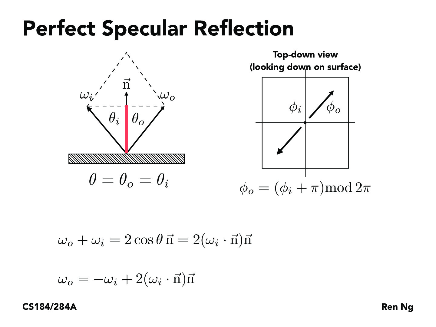
Just as in Part 1 of this assignment, sampling BSDFs take in an outgoing ray direction and sample an incoming ray direction, returning a value that represents how much light should be reflected between these directions. Since a perfectly specular material reflects all rays across the surface normal, I used the reflection equation, shown above, to “sample” incoming ray directions.

The maximum ray depth for the renderer must be greater than one in order for the reflective surface to work. Otherwise, in the case of a ray depth of 1, the mirror will only reflect if the reflected ray hits a light, since it will not be able to capture light contributions from objects that light ray bounced off of. In the case of a ray depth of 0, nothing will render outside of the lights.

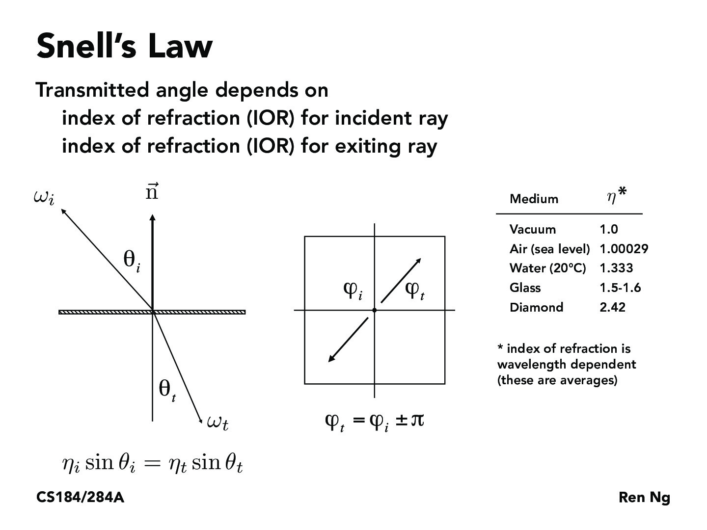
Unlike reflections, where rays bounce off a surface, refractive surfaces bend rays of light into the surface based off of the indices of refraction (IORs) of the incoming medium and the outgoing medium. Snell’s law is a law that describes the relationship between an incident ray and an exiting ray. I implemented Snell’s law in order to model refractions.

Since glass surfaces both reflect and refract for many light rays, implementing the glass material BSDF requires modeling the ratio of reflection energy to the refraction energy. It was suggested that we use Schlick’s approximation to determine the ratio between reflection energy and refraction energy when sampling the BSDF.

I increased the maximum ray depth across these renders. When the maximum ray depth is 0, as before, only the lights render since only camera rays that directly hit a light will return something other than black. As mentioned previously, a max ray depth of 1 only shows reflected lights, since reflected rays that hit objects that do not emit light will not return any color contribution, since this is not considered in one-bounce illumination.

With two bounces, the mirror material successfully captures a reflection of its surroundings, and the glass material begins to have some visible reflection and refraction. Examining the mirror material reveals that the reflected scenery does not perfectly mirror its surroundings–the ceiling and the glass sphere are much darker, since objects that appear in reflections have light contributions from with one less bounce than when they are rendered directly. The render is noticeably noisier, since allowing more bounces complicates the path of lights through a scene.

When the number of bounces increase, the appearance of the reflected surroundings is more accurate since the lighting in many areas converges over many bounces. The glass material also gets noticeably brighter, since increasing max ray depth allows more light to pass through the glass. When max ray depth is 4 or greater, a bright spot can be seen on the right side of the image on the blue wall–this spot is the result of light rays refracting through the sphere and hitting the wall. This path takes at least 4 bounces to simulate, which is why it is not present in previous renders.

Part 7: Microfacet Material

In this stage, I implemented a BSDF for a Microfacet material. These materials are not perfectly specular, with some isotropic roughness that changes how they reflect light.

The Microfacet BRDF was provided, split up into multiple parts. The main components of this function, as described by the spec, are as follows: “F is the Fresnel term, G is the shadowing-masking term, and D is the normal distribution function (NDF).”

The Beckmann NDF is used to distribute the microfacets’ normals, with the alpha term controlling the roughness of the object. Each microfacet is treated as perfectly specular along the half vector h.

The Fresnel term for microfacet surfaces is more complex than it was for refractive surfaces, since material defines air-conductor surfaces. The provided equations are above, and they approximate the true Freshenl term by finding the Fresnel term for the R, G, and B channels. eta and k define the indices of refraction for conductors.

The final step for this part was to implement a new importance sampling distribution, since cosine-weighted hemisphere sampling is usually inefficient for microfacet materials. This function was based off the shape of the Beckmann NDF.

With a = 0.005, the metal is extremely smooth, with no strong highlights and visible reflections from the walls. Increasing a to 0.05 causes more noticeable highlights to appear on the dragon, though the reflection is still prominent. When a = 0.25, the surface is much less smooth, with reflection only visible in certain parts as the highlights grow larger. Finally, when a is 0.5, the surface is rough to the point of appearing diffuse in some areas, with a large areas of reflected light scattered around the surface.

The two renders above demonstrate why the importance sampling was necessary to improve the quality of the render. With cosine hemisphere sampling, the reflected light will only count if the sampling rays happen to align with the half vectors of the microfacets. As a result, there are many more black and grainy regions on the bunny on the left. In comparison, importance sampling on the Beckmann NDF function allows the path tracer to more accurately represent the microfacet material.

Using this website, I found the IORs for cobalt to input into the microfacet model. This demonstrates the versatility of the microfacet model, as it is able to physically simulate a wide variety of materials.